The following is the short description of the full small end to end data science project I chose for myself. I always wanted to play with text data, so I chose to create my own corpus. I will use it later to apply some machine learning on top of it. Take a look at how do I predict a category of some blog posts.
Goal
Recently I learn about Machine Learning (ML). There are lots of possible areas of use: analyzing video, images, speech and text. The last one seems to be the most appealing to me. Online content grows every day. We have too much to read. Natural Language Processing (NLP) is a data science response to this problem. The content of my small project comes from a great developer community blog: dev.to. To show basic ML I will guess the tag based on the dev.to post content. Thus, I will run supervised learning. In simple words: I am pasting the content of a post and it should tell me is this about “java” or maybe “python”. The effect of my work is a web app, so feel free to play with it here. For the sake of simplicity, I used 4 major categories only. Take a look on this life demo gif:
Corpus
What is a corpus? In the NLP world, it is a group of documents. We will analyze these documents later on. Doing any ML project you have to start with something to analyze. With some data. In NLP you have to get some texts. It is not obligatory to scrape them from some internet portal. You can start with built-in corpora as these being part of nltk library described here. In my case, I want use dev.to data, so I will use API they expose. I will create my own corpus. The process of data acquisition is visible as part of my GitHub project here. Doing it with Python is so easy, I can use great libraries, such as BeautifulSoap and requests.
BoW
The BoW acronym stands for Bag of Words. This is a simple way of vectorization of text. Its name comes from the idea of having a bag where we put all the words. We don’t care how are they ordered. We just need to vectorize our text. This is a prerequisite before applying any ML algorithm on text. So how does this vector look like for a simple sentence? Taking a CountVectorizer available as part of Scikit Learn library let us see how does it transform text to vector.
sentences = [
  "I like playing the violin",
  "Playing football is nice",
  "How do you like playing football?"
]

from sklearn.feature_extraction.text import CountVectorizer
import operator
vectorizer = CountVectorizer()
X = vectorizer.fit_transform(sentences)
vocabulary = vectorizer.vocabulary_.items()
vocabulary_sorted = sorted(vocabulary, key=operator.itemgetter(1))
print("vocabulary is:")
print(vocabulary_sorted)
print("matrix resulted is:")
print(X.toarray())
The result would be:
vocabulary is:
[('do', 0), ('football', 1), ('how', 2), ('is', 3), ('like', 4), ('nice', 5), ('playing', 6), ('the', 7), ('violin', 8), ('you', 9)]
matrix resulted is:
[[0 0 0 0 1 0 1 1 1 0]
 [0 1 0 1 0 1 1 0 0 0]
 [1 1 1 0 1 0 1 0 0 1]]
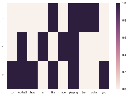
And let us see how does it look like when we visualize it as a heat map:
As we will produce a model soon we want to make it of good quality. We will perform a Tf-Idf (Term Frequency - Inverse Document Frequency) transformation. It means we take into consideration how frequent the word is in a document (TF) and how rare it is among other documents (IDF). Applying this transformation in sklearn results in a matrix little different from what we saw before:
vocabulary is:
[('do', 0), ('football', 1), ('how', 2), ('is', 3), ('like', 4), ('nice', 5), ('playing', 6), ('the', 7), ('violin', 8), ('you', 9)]
TfIdf matrix resulted is:
[[0.         0.         0.         0.         0.44451431 0.
  0.34520502 0.5844829  0.5844829  0.        ]
 [0.         0.44451431 0.         0.5844829  0.         0.5844829
  0.34520502 0.         0.         0.        ]
 [0.4711101  0.35829137 0.4711101  0.         0.35829137 0.
  0.27824521 0.         0.         0.4711101 ]]
And the visualization
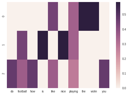
The output matrix is little different now. It is because we care how often terms occur in the whole data set. In our case TfIdf promotes rare ones like violin and deprecates the popular, like playing.
Machine Learning
Having vector ready we can apply math on top of that. In supervised learning we have to find a function that matches input vector X with label y. Having structure and kind of data we process there is a need to apply the correct algorithm, not just a random one. If you’re facing this problem find this sklearn cheatsheet. In my case, I am doing the classification of textual data. I found many experienced data scientists tend to use Naive Bayes for that. After several trials I found it useful, too. You can check my notebook here. Remember, with textual data we use the Multinomial and not the Gaussian algorithm. So there is a snippet from the model training process.
import pandas as pd
from sklearn.naive_bayes import MultinomialNB
from sklearn.model_selection import train_test_split

def train_naivebayes(X, y):
  X_train, X_test, y_train, y_test = train_test_split(X, y, random_state=0)
  bayes = MultinomialNB()
  bayes_model = bayes.fit(X_train, y_train)
  y_pred = bayes_model.predict(X_test)
Please find the full codebase in my repo.
Deploy
Once your model is ready there is a time to share it with others! You can do it with Azure or AWS. They usually have ready-to-use Docker containers where you just have to put your model inside, and they magically expose it as a REST service. However, the 1st time I expose some model I wanted to have everything under control. This is why I decided to build my model inside of a web application myself. It is as easy as serializing building blocks to files and then uploading these files to a server. You can go there and check my app deployed.
Lessons learned
I do not think the project is perfect. I measured the accuracy of the model and it is around 80%. To have better results we could:
- use another algorithm, f.e. ensemble algorithm, or tune the existing one
- have more data than hundreds of entries (more data always means: better)
- clean data better
I am happy to see how a nice experience working with data with sklearn was. Python provides a must-have ML tool belt. I also tasted the full stack of the ML problem. I collected, analyzed, fitted model and finally deployed it.